Newton method to solve nonlinear circuits
In this tutorial we will see how ForwardModeAD can be used to easily implement the Newton method to solve nonlinear equations. As an application, we will demo how this can be used to solve nonlinear electric circuits.
Newton method
Suppose we want to solve a nonlinear equation \(f(x)=0\). The Newton rule is an iterative algorithm that starts with an initial guess of the root \(x_0\) and uses the following update rule
In general, but with some pathological exceptions, the update rule will converge quadratically to a root of the function.
As we need the derivative of the function, the algorithm is easily implemented with ForwardModeAD.
We also need a stopping criteria for the update rule, here we choose to stop when \(|f(x_n)|<tol\). Where \(tol\) is a chosen tolerance.
Now we have everything we need to implement, the algorithm, let us demo it by finding the root of the function
using initial guess \(x_0=0.5\) and tolerance \(10^{-6}\).
use ForwardModeAD;

proc f(x) {
    return exp(-x) * sin(x) - log(x);
}

var tol = 1e-6, // tolerance to find the root
    cnt = 0, // to count number of iterations
    x0 = initdual(0.5), // initial guess
    valder = f(x0); // initial function value and derivative

while abs(value(valder)) > tol {
    x0 -= value(valder) / derivative(valder);
    valder = f(x0);
    cnt += 1;
    writeln("Iteration ", cnt, " x = ", value(x0), " residual = ", value(valder));
}
Iteration 1 x = 1.05953 residual = 0.244472
Iteration 2 x = 1.28662 residual = 0.0131033
Iteration 3 x = 1.3002 residual = 4.13149e-05
Iteration 4 x = 1.30025 residual = 4.13897e-10
As you can see, the algorithm quickly converges to \(x \approx 1.30025\), which is the correct root.
Nonlinear circuit example
Solving nonlinear equations is very common in most if not all scientific computing applications. To make our example more concrete, let us demo how the previous algorithm can be used to analyze the following nolinear circuit, using values \(R=1~\textrm{k}\Omega\) and \(E=5~\textrm{V}\).
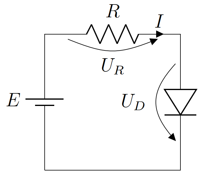
The resistor is modeled via Ohm law \(U_R=RI\) and the diode via Schockley equation \(I=I_S\left(e^\frac{V_D}{V_T}-1\right)\), with \(I_S\approx10^{-12}\) and \(V_T\approx25~\textrm{mV}\).
By Kirchoff voltage law we have
Subsituting the previous values and equations we get
this can be now solved with our previously developed Newton method
proc g(vd) {
    return 1e-9 * (exp(40 * vd) - 1) + vd - 5;
}

var Vd = initdual(0.0), // voltage initial guess
    Id = g(Vd), // initial current value
    tol = 1e-6; // tolerance

while abs(value(Id)) > tol {
  Vd -= value(Id) / derivative(Id);
  Id = g(Vd);
}

writeln("V = ", value(Vd), "\n");
x0 = 0.555374
which is indeed a typical voltage value for a diode.
Newton method in higher dimension
In the previous example we considered one equation in one unknown. The Newton method can also be applied to the case of \(n\) equations in \(n\) unknowns, that is to solve the nonlinear system of equations \(F(X)=\mathbf{0}\) with \(F:\mathbb{R}^n\rightarrow\mathbb{R}^n\).
The update rule for this higher dimension problem becomes
Note that the derivative has now been replaced by the Jacobian. Note also that the quantity \(J_F(X_n)^{-1}F(X_n)\) can be computed by solving the linear system
\(J_F(X_n)Y=F(X_n)\), using the function solve from the LinearAlgebra module, no need to explicitly invert the matrix.
Finally, in 1D our stopping criterion was \(|x_n|<tol\) for some predefined tolerance. In higher dimensions this generalizes to \(\Vert X_n\Vert<tol\),
where \(\Vert\cdot\Vert\) is some vector norm. In this example we choose the classical Euclidean norm, computed with the Chapel norm function from LinearAlgebra.
We now have all the ingredients to program the higher dimension Newton method, let’s do it with the following example
using as initial guess \(X_0=[3, 3]\).
use LinearAlgebra; // needed for solve and norm

proc F(x) {
    return [log(x[0]) - x[1] + 0.5, x[0]**2 - x[0]*x[1] - 0.7];
}

var cnt = 0, // to count number of iterations
    tol = 1e-6, // tolerance
    X0 = [3.0, 3.0], // initial guess
    valjac = F(initdual(X0)), // initial function value and derivative
    res = norm(value(valjac)); // initial residue residual ||F(X_0)||

writeln("Iteration ", cnt, " x = ", X0, " residual = ", res);

while res > tol {
    X0 -= solve(jacobian(valjac), value(valjac))
    valjac = F(initdual(X0));
    res = norm(value(valjac));
    cnt += 1;
    writeln("Iteration ", cnt, " x = ", X0, " residual = ", res);
}
Iteration 0 x = 3.0 3.0 residual = 1.56649
Iteration 1 x = 1.24792 1.01459 residual = 0.503036
Iteration 2 x = 1.33736 0.79315 residual = 0.0279132
Iteration 3 x = 1.3021 0.764332 residual = 0.000420461
Iteration 4 x = 1.30128 0.763349 residual = 2.39082e-07